2.14. Applying a field that changes both in time and in space
2.14.1. Idea: pass simulation object to field-setting function
You can simulate an applied field which both changes in space and
time: this may be useful to mimic the effect of a write head on the
magnetic grains of an hard disk while the head is moving. The way we
do this is by changing the applied field every delta_t
picoseconds. This means that the applied field won’t change
continuously in time: it will be piecewise constant in time (but, in
general, it can be non uniform in space). You can do something like:
import math

def set_H(sim):
  width = 10.0        # nm
  v = 100.0           # nm/ns == m/s
  H_amplitude = 0.5e6 # A/m

  t = float(sim.time/SI(1e-9, 's')) # get the time in ns
  center = (v*t, 0, 0) # center of the applied field region
  def H(r):
    x, y, z = [ri/1e-9 - ci for ri, ci in zip(r, center)]
    factor = H_amplitude*math.exp(-(x*x + y*y + z*z)/(width*width))
    return [factor, factor, factor]

  sim.set_H_ext(H, unit=SI('A/m'))

sim.relax(do=[(set_H, every('time', SI(50e-12, 's'))),
              ('exit', at('time', SI(1000e-12, 's')))])
The function set_H is called every 50 ps and does the following: it
sets a new field from the function H(r). This function sets a field
which directed along the direction [1, 1, 1] and almost vanishes
outside a sphere with radius ~ 30.0 nm. The center of this sphere
moves along the direction [1, 0, 0] with velocity 100 nm/ns, thus
simulating the motion of a write head in a hard disk. Obviously the
piece of code is not complete, it shows only the technique in order to
have a field changing in time and space. For a complete example see
the next section.
2.14.2. Complete example: simple moving write-head example
Here is a simulation of five cubes made of cobalt and a write-head which moves on the top of the cubes and applies a time-varying field in order to change their magnetisation. At the beginning the magnetisation of all the cubes is pointing in the [0, 0, 1] direction. After the write-head has passed over the cubes, the magnetisation of cube 1, 3 and 5 are switched in the opposite direction, while cube 2 and 4 have unchanged magnetisation. This is possible because the write-head field, which is space-dependent (being intense only inside a sphere of radius 15-20 nm), changes also in time. It indeed translates in space, but also change in intensity, being directed in the [0, 0, -1] direction when the sphere is at the center of cube 1, 3 and 5 and in the [0, 0, 1] direction when the center of the sphere is in cube 2 and 4.
Here is the geo file used to generate the mesh (Netgen):
<pre>
algebraic3d

# cubes
solid cube1 = orthobrick (    0, 0, 0;  20.0, 20.0, 20.0) -maxh = 2;
solid cube2 = orthobrick ( 30.0, 0, 0;  50.0, 20.0, 20.0) -maxh = 2;
solid cube3 = orthobrick ( 60.0, 0, 0;  80.0, 20.0, 20.0) -maxh = 2;
solid cube4 = orthobrick ( 90.0, 0, 0; 110.0, 20.0, 20.0) -maxh = 2;
solid cube5 = orthobrick (120.0, 0, 0; 140.0, 20.0, 20.0) -maxh = 2;

tlo cube1;
tlo cube2;
tlo cube3;
tlo cube4;
tlo cube5;
And here is the full listing of the example:
from nmag.common import *
import math

# Define magnetic material (data from OOMMF materials file)
mat_Co = MagMaterial(name="Co",
                     Ms=SI(1400e3, "A/m"),
                     exchange_coupling=SI(30e-12, "J/m"),
                     anisotropy=uniaxial_anisotropy(axis=[0, 0, 1],
                                                    K1=SI(520e3, "J/m^3")))
sim = Simulation()
sim.load_mesh("cubes.nmesh.h5",
              [('cube1', mat_Co), ('cube2', mat_Co), ('cube3', mat_Co),
               ('cube4', mat_Co), ('cube5', mat_Co)],
              unit_length=SI(1e-9, 'm'))

sim.set_m([0, 0, 1])

sim.relax(save=[('fields', at('convergence'))])

t0 = [sim.time]

def set_H(sim):
    t = float((sim.time - t0[0])/SI(1e-9, 's'))  # get time in ns
    width = 10.0                                 # nm
    v = 25.0                                     # nm/ns = m/s
    H_amplitude = 4.0e6*math.sin(math.pi*t)      # A/m
    center = (v*t, 20, 10)
    print "CENTER IN", center
    def H(r):
        x, y, z = [ri/1e-9 - ci for ri, ci in zip(r, center)]
        factor = H_amplitude*math.exp(-(x*x + y*y + z*z)/(width*width))
        return [0, 0, -factor]

    sim.set_H_ext(H, unit=SI('A/m'))

set_H(sim)

sim.set_params(stopping_dm_dt=0*degrees_per_ns)

sim.relax(save=[('fields', every('time', SI(200e-12, 's'), first=t0[0]))],
          do=[(set_H, every('time', SI(50e-12, 's'), first=t0[0])),
              ('exit', at('time', SI(6000e-12, 's')))])
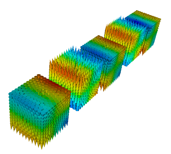
Here is the magnetisation at the beginning of the simulation, after the first relax command (whose purpose is just to find the zero field magnetisation configuration):
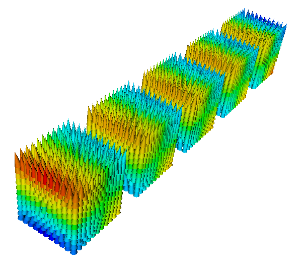
and here is the magnetisation after the write-head has passed over the cubes: