2.7. Example: Manipulating magnetisation
There are two basic techniques to modify the magnetisation: on the one hand, we can use the set_m method to replace the current magnetisation configuration with a new one. We can use set_m to specify both homogeneous (see Setting the initial magnetisation) and non-homogeneous magnetisations (see the Spin-waves example). Alternatively, we can selectively change magnetic moments at individual mesh sites. This example demonstrates how to use the latter technique.
The basics of this system are as in Example: Demag field in uniformly
magnetised sphere: we study a ferromagnetic sphere with initially
homogeneous magnetisation. The corresponding script file is
sphere_manipulate.py
import nmag
from nmag import SI

# Create simulation object
sim = nmag.Simulation()

# Define magnetic material
Py = nmag.MagMaterial(name="Py",
                      Ms=SI(1e6, "A/m"),
                      exchange_coupling=SI(13.0e-12, "J/m"))

# Load mesh
sim.load_mesh("sphere1.nmesh.h5", [("sphere", Py)], unit_length=SI(1e-9, "m"))

# Set initial magnetisation
sim.set_m([1, 0, 0])

# Set external field
sim.set_H_ext([0, 0, 0], SI("A/m"))

# Save and display data in a variety of ways
# Step 1: save all fields spatially resolved

sim.save_data(fields='all')

# Step 2: sample demag field through sphere
for i in range(-10, 11):
    x = i*1e-9                      # position in metres
    H_demag = sim.probe_subfield_siv('H_demag', [x, 0, 0])
    print "x =", x, ": H_demag = ", H_demag

# Step 3: sample exchange field through sphere
for i in range(-10, 11):
    x = i*1e-9                      # position in metres
    H_exch_Py = sim.probe_subfield_siv('H_exch_Py', [x, 0, 0])
    print "x =", x, ": H_exch_Py = ", H_exch_Py


# Now modify the magnetisation at position (0,0,0) (this happens to be
# node 0 in the mesh) in steps 4 to 6:

# Step 4: request a vector with the magnetisation of all sites in the mesh
myM = sim.get_subfield('m_Py')

# Step 5:  We modify the first entry:
myM[0] = [0, 1, 0]

# Step 6: Set the magnetisation to the new (modified) values
sim.set_m(myM)

# Step 7: saving the fields again (so that we can later plot the demag
# and exchange field)
sim.save_data(fields='all')

# Step 8: sample demag field through sphere (as step 2)
for i in range(-10, 11):
    x = i*1e-9                      # position in metres
    H_demag = sim.probe_subfield_siv('H_demag', [x, 0, 0])
    print "x =", x, ": H_demag = ", H_demag

# Step 9: sample exchange field through sphere (as step 3)
for i in range(-10, 11):
    x = i*1e-9                      # position in metres
    H_exch_Py = sim.probe_subfield_siv('H_exch_Py', [x, 0, 0])
    print "x =", x, ": H_exch_Py = ", H_exch_Py
To execute this script, we have to give its name to the nsim executable, for example (on linux):
$ nsim sphere_manipulate.py
After having created the simulation object, defined the material, loaded the mesh, set the initial magnetisation and the external field, we save the data the first time (Step 1).
We could visualise the magnetisation and all other fields as described in Example: Demag field in uniformly magnetised sphere, and would obtain the same figures as shown in section Saving spatially resolved data.
In step 2, we probe the demag field at positions along a line going from [-10,0,0]nm to [10,0,0]nm, and then print the values. This produces the following output:
x = -1e-08 : H_demag =  None
x = -9e-09 : H_demag =  [-329656.18892701436, 131.69946810517845, 197.13873034397167]
x = -8e-09 : H_demag =  [-329783.31649797881, 68.617197264295427, 140.00328871543459]
x = -7e-09 : H_demag =  [-329842.17628131888, 183.37401011699876, 163.01612229436262]
x = -6e-09 : H_demag =  [-329904.84956877632, 133.62473797637142, 74.090532749764847]
x = -5e-09 : H_demag =  [-329974.43178624194, 85.517390832982983, -13.956465964930704]
x = -4e-09 : H_demag =  [-330002.69224229571, 64.187663119270084, -30.832135394870004]
x = -3e-09 : H_demag =  [-330006.79488959321, 25.479055440690821, -61.958073893954818]
x = -2e-09 : H_demag =  [-330020.18327401817, 11.70722487517595, -58.143562276077219]
x = -1e-09 : H_demag =  [-330025.52325345919, -5.7120648683347452, -52.237341988696294]
x = 0.0    : H_demag =  [-330028.67095553532, -25.707310077918752, -46.346108473560378]
x = 1e-09  : H_demag =  [-330058.98559210222, -37.699378078580203, -41.167364094137213]
x = 2e-09  : H_demag =  [-330089.30022866925, -49.691446079241658, -35.988619714714041]
x = 3e-09  : H_demag =  [-330145.36618529289, -63.819285767062581, -22.213920341440794]
x = 4e-09  : H_demag =  [-330220.13307247689, -76.54950394725968, -5.0509172407556262]
x = 5e-09  : H_demag =  [-330298.69089200837, -90.534514175273259, 13.57279800234617]
x = 6e-09  : H_demag =  [-330375.34327985492, -117.01128011426778, 35.262477275758371]
x = 7e-09  : H_demag =  [-330415.38940687838, -123.68558207391983, 60.580352625726341]
x = 8e-09  : H_demag =  [-330474.37719032855, -112.22952205433305, 106.13032196062491]
x = 9e-09  : H_demag =  [-330499.64039893239, -69.97070465326442, 160.41688110297264]
x = 1e-08  : H_demag =  [-330518.649930441, -26.536490670368085, 212.32392103651733]
The data is approximately 1/3 Ms = 333333 (A/m) in the direction of the magnetisation, and approximately zero in the other directions, as we would expect in a homogeneously magnetised sphere. The deviations we see are due to (i) the shape of the sphere not being perfectly resolved (ie we actually look at the demag field of a polyhedron) and (ii) numerical errors.
In step 3, we probe the exchange field along the same line. The exchange field is effectively zero because the magnetisation is pointing everywhere in the same direction:
x = -1e-08 : H_exch_Py =  None
x = -9e-09 : H_exch_Py =  [-1.264324643856989e-09, 0.0, 0.0]
x = -8e-09 : H_exch_Py =  [-2.0419540595507732e-10, 0.0, 0.0]
x = -7e-09 : H_exch_Py =  [-1.4334754136843496e-09, 0.0, 0.0]
x = -6e-09 : H_exch_Py =  [-2.7214181426130964e-10, 0.0, 0.0]
x = -5e-09 : H_exch_Py =  [1.6323042074911775e-09, 0.0, 0.0]
x = -4e-09 : H_exch_Py =  [-1.6243345875473033e-09, 0.0, 0.0]
x = -3e-09 : H_exch_Py =  [-5.6526341264934703e-09, 0.0, 0.0]
x = -2e-09 : H_exch_Py =  [-6.1145979552370084e-09, 0.0, 0.0]
x = -1e-09 : H_exch_Py =  [-3.0929969691649876e-09, 0.0, 0.0]
x = 0.0    : H_exch_Py =  [9.2633407053741312e-10, 0.0, 0.0]
x = 1e-09  : H_exch_Py =  [1.9476821552904271e-09, 0.0, 0.0]
x = 2e-09  : H_exch_Py =  [2.9690302400434413e-09, 0.0, 0.0]
x = 3e-09  : H_exch_Py =  [2.6077357277001043e-09, 0.0, 0.0]
x = 4e-09  : H_exch_Py =  [1.5836815585162886e-09, 0.0, 0.0]
x = 5e-09  : H_exch_Py =  [1.6602158583197139e-09, 0.0, 0.0]
x = 6e-09  : H_exch_Py =  [1.8844573960991853e-09, 0.0, 0.0]
x = 7e-09  : H_exch_Py =  [-6.2460015649740799e-09, 0.0, 0.0]
x = 8e-09  : H_exch_Py =  [-1.1231714572170603e-08, 0.0, 0.0]
x = 9e-09  : H_exch_Py =  [-7.3643182171284044e-09, 0.0, 0.0]
x = 1e-08  : H_exch_Py =  [-3.4351784609779937e-09, 0.0, 0.0]
Note that the subfield name we are probing for the exchange field is
H_exch_Py whereas the subfield name we used to probe the demag
field is H_demag (without the extension _Py. The reason for
this is that the exchange field is a something that is associated with
a particular material (here Py) whereas there is only one demag field
that is experienced by all materials (see also Fields and subfields).
2.7.1. Modifying the magnetisation
In step 4, we use the get_subfield command. This will return a (NumPy) array that contains one 3d vector for every Site of the finite element mesh.
In step 5, we modify the first entry in this array (which has index
0), and set its value to [0,1,0]. Whereas the magnetisation is
pointing everywhere in [1,0,0] (because we have used the set_m
command in the very beginning of the program, it is now pointing in
the [0,1,0] at site 0.
The information, which site corresponds to which entry in the data vector, that we have obtained using get_subfield, can be retrieved from get_subfield_sites. Correspondingly, the position of the sites can be obtained using get_subfield_positions.
We now need to set this modified magnetisation vector (Step 6) using the set_m command.
If we save the data again to the file (Step 7), we can subsequently
convert this to a vtk file (using, for example, nmagpp --vtk data
sphere_manipulate) and visualise with MayaVi:
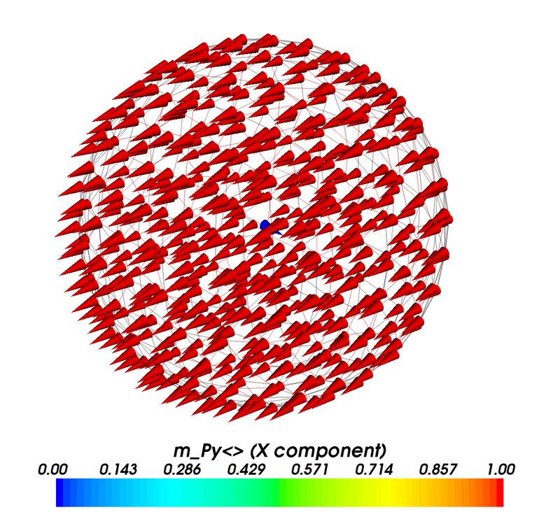
We can see one blue cone in the centre of the sphere - this is the one site that he have modified to point in the y-direction (whereas all other cones point in the x-direction).
As before, we can probe the fields along a line through the center of the sphere (Step 8). For the demag field we obtain:
x = -1e-08 : H_demag =  None
x = -9e-09 : H_demag =  [-333816.99138074159, -1884.643376396662, 16.665519199152595]
x = -8e-09 : H_demag =  [-334670.87148225965, -2293.608410913705, -102.38526828192296]
x = -7e-09 : H_demag =  [-335258.77403632947, -3061.1708540342884, -532.73877752122235]
x = -6e-09 : H_demag =  [-339506.72150998382, -5316.1506383768137, -969.36630578549921]
x = -5e-09 : H_demag =  [-344177.83909963415, -8732.9787600552572, -1610.433091871927]
x = -4e-09 : H_demag =  [-344725.75257842313, -16708.164927667149, -5224.2484897904633]
x = -3e-09 : H_demag =  [-337963.49070659198, -24567.078937669514, -3321.016613832679]
x = -2e-09 : H_demag =  [-321612.85117992124, -30613.873989917105, -1385.6383061516099]
x = -1e-09 : H_demag =  [-298312.3363571504, -41265.117003123923, 636.60703829516081]
x = 0.0    : H_demag =  [-273449.78240732534, -52534.176864875568, 2793.5027588779139]
x = 1e-09  : H_demag =  [-293644.21931918303, -39844.049389551074, 4310.6449471266505]
x = 2e-09  : H_demag =  [-313838.65623104072, -27153.921914226579, 5827.7871353753881]
x = 3e-09  : H_demag =  [-330296.09687372146, -21814.293451835449, 5525.7290665358933]
x = 4e-09  : H_demag =  [-343611.94111195666, -18185.932406317523, 4931.5464761658959]
x = 5e-09  : H_demag =  [-348062.40814087034, -11029.603829202088, 3781.8263522408147]
x = 6e-09  : H_demag =  [-342272.36888512014, -6604.210117819096, 50.151907623841332]
x = 7e-09  : H_demag =  [-338716.66400897497, -3860.7761876767272, 485.90273674867018]
x = 8e-09  : H_demag =  [-335656.89887674141, -2610.0345208853882, 586.74812908870092]
x = 9e-09  : H_demag =  [-334985.59512328985, -2169.9546280837162, 542.76746044672041]
x = 1e-08  : H_demag =  [-334441.59096545313, -1634.8337299563193, 627.17874011463311]
The change of the magnetisation at position [0,0,0] from [1,0,0] to [0,1,0] has reduced the x-component of the demag field somewhat around x=0, and has introduced a significant demag field in the -y direction around x=0.
Looking at the exchange field (Step 9):
x = -1e-08 : H_exch_Py =  None
x = -9e-09 : H_exch_Py =  [-1.264324643856989e-09, 0.0, 0.0]
x = -8e-09 : H_exch_Py =  [-2.0419540595507732e-10, 0.0, 0.0]
x = -7e-09 : H_exch_Py =  [-1.4334754136843496e-09, 0.0, 0.0]
x = -6e-09 : H_exch_Py =  [-2.7214181426130964e-10, 0.0, 0.0]
x = -5e-09 : H_exch_Py =  [1.6323042074911775e-09, 0.0, 0.0]
x = -4e-09 : H_exch_Py =  [-153858.81305452777, 153858.81305452611, 0.0]
x = -3e-09 : H_exch_Py =  [-972420.67935341748, 972420.67935341166, 0.0]
x = -2e-09 : H_exch_Py =  [-2445371.8369108676, 2445371.8369108611, 0.0]
x = -1e-09 : H_exch_Py =  [5283169.701234119, -5283169.7012341227, 0.0]
x = 0.0    : H_exch_Py =  [15888993.991894867, -15888993.991894867, 0.0]
x = 1e-09 :  H_exch_Py =  [8434471.7912872285, -8434471.7912872266, 0.0]
x = 2e-09 :  H_exch_Py =  [979949.59067958547, -979949.59067958279, 0.0]
x = 3e-09 :  H_exch_Py =  [-1112837.3087986181, 1112837.3087986207, 0.0]
x = 4e-09 :  H_exch_Py =  [-193877.66176242317, 193877.6617624248, 0.0]
x = 5e-09 :  H_exch_Py =  [1.6602158583197139e-09, 0.0, 0.0]
x = 6e-09 :  H_exch_Py =  [1.8844573960991853e-09, 0.0, 0.0]
x = 7e-09 :  H_exch_Py =  [-6.2460015649740799e-09, 0.0, 0.0]
x = 8e-09 :  H_exch_Py =  [-1.1231714572170603e-08, 0.0, 0.0]
x = 9e-09 :  H_exch_Py =  [-7.3643182171284044e-09, 0.0, 0.0]
x = 1e-08 :  H_exch_Py =  [-3.4351784609779937e-09, 0.0, 0.0]
We can see that the exchange field is indeed very large around x=0.
Note that one of the fundamental problem of micromagnetic simulations is that the magnetisation must not vary significantly from one site to another. In this example, we have manually violated this requirement only to demonstrate how the magnetisation can be modified, and to see that this is reflected in the dependant fields (such as demag and exchange) immediately.