2.12. Example: Arbitrary Anisotropy
In this example we discuss
the script coin.py
which shows how the user can include in his simulations
a customised magnetic anisotropy.
2.12.1. Arbitrary anisotropy simulation script
import nmag
from nmag import SI, every, at
from nsim.si_units import si
import math

# Create simulation object (no demag field!)
sim = nmag.Simulation(do_demag=False)

# Function to compute the scalar product of the vectors a and b
def scalar_product(a, b): return a[0]*b[0] + a[1]*b[1] + a[2]*b[2]

# Here we define a function which returns the energy for a uniaxial
# anisotropy of order 4.
K1 = SI(43e3, "J/m^3")
K2 = SI(21e3, "J/m^3")
axis = [0, 0, 1]        # The (normalised) axis
def my_anisotropy(m):
    a = scalar_product(axis, m)
    return -K1*a**2 - K2*a**4

my_material = nmag.MagMaterial(name="MyMat",
                               Ms=SI(1e6, "A/m"),
                               exchange_coupling=SI(10e-12, "J/m"),
                               anisotropy=my_anisotropy,
                               anisotropy_order=4)

# Load the mesh
sim.load_mesh("coin.nmesh.h5", [("coin", my_material)], unit_length=SI(1e-9, "m"))

# Set the magnetization
sim.set_m([-1, 0, 0])

# Compute the hysteresis loop
Hs = nmag.vector_set(direction=[1.0, 0, 0.0001],
                     norm_list=[-0.4, -0.35, [], 0, 0.005, [], 0.15, 0.2, [], 0.4],
                     units=si.Tesla/si.mu0)

sim.hysteresis(Hs, save=[('fields', 'averages', at('convergence'))])
We simulate the hysteresis loop for a ferromagnetic thin disc, where the field is applied orthogonal to the axis of disc. This script includes one main element of novelty, which concerns the way the magnetic anisotropy is specified. In previous examples we found lines such as:
my_material = nmag.MagMaterial(name="MyMat",
                               Ms=SI(1e6, "A/m"),
                               exchange_coupling=SI(10e-12, "J/m"),
                               anisotropy=nmag.uniaxial_anisotropy(axis=[0, 0, 1],
                                                                   K1=SI(43e3, "J/m^3"),
                                                                   K2=SI(21e3, "J/m^3")))
where the material anisotropy was specified using the provided functions
nmag.uniaxial_anisotropy (uniaxial_anisotropy) and nmag.cubic_anisotropy (cubic_anisotropy).
In this example we are using a different approach to define the anisotropy.
First we define the function my_anisotropy, which returns the energy density
for the magnetic anisotropy:
# Here we define a function which returns the energy for a uniaxial
# anisotropy of order 4.
K1 = SI(43e3, "J/m^3")
K2 = SI(21e3, "J/m^3")
axis = [0, 0, 1]        # The (normalised) axis
def my_anisotropy(m):
    a = scalar_product(axis, m)
    return -K1*a**2 - K2*a**4
Note that the function returns a SI object with units “J/m^3” (energy density).
The reader may have recognised the familiar expression for the uniaxial anisotropy:
in fact the two code snippets we just presented are defining exactly the same
anisotropy, they are just doing it in different ways.
The function scalar_product, which we have used in the second code snippet
just returns the scalar product of two three dimensional vectors a and b
and is defined in the line above:
def scalar_product(a, b): return a[0]*b[0] + a[1]*b[1] + a[2]*b[2]
The function my_anisotropy has to be specified in the material definition:
instead of passing anisotropy=nmag.uniaxial_anisotropy(...)
we just pass anisotropy=my_anisotropy to the material constructor:
my_material = nmag.MagMaterial(name="MyMat",
                               Ms=SI(1e6, "A/m"),
                               exchange_coupling=SI(10e-12, "J/m"),
                               anisotropy=my_anisotropy,
                               anisotropy_order=4)
An important point to notice is that here we also provide an anisotropy order.
To understand what this number is, we have to explain briefly what is going on
behind the scenes. |nsim| calculates the values of the user provided function
for an appropriately chosen set of normalised vectors,
it then finds the polynomial in mx, my and mz
(the components of the normalised magnetisation) of the specified order,
which matches the sampled values.
The strength of this approach stands in the fact that the user has to provide just the energy density for the custom anisotropy. |nsim| is taking care of working out the other quantities which are needed for the simulation, such as the magnetic field resulting from the provided anisotropy energy, which would require a differentiation of the energy with respect to the normalised magnetisation.
However the user must be sure that the provided function can be expressed
by a polynomial of the specified order in mx, my and mz.
In the present case we are specifying anisotropy_order=4 because the energy
for the uniaxial anisotropy can be expressed as a 4th-order polynomial
in mx, my and mz.
In some cases the user may find useful to know that the functions
nmag.uniaxial_anisotropy and nmag.cubic_anisotropy
can be added: the resulting anisotropy will have as energy
the sum of the energies of the original anisotropies.
2.12.2. The result
The steps involved to extract and plot the data for the simulation discussed
in the previous section should be familiar to the user at this point of the manual.
We then just show the graph obtained from the results
of the script coin.py.
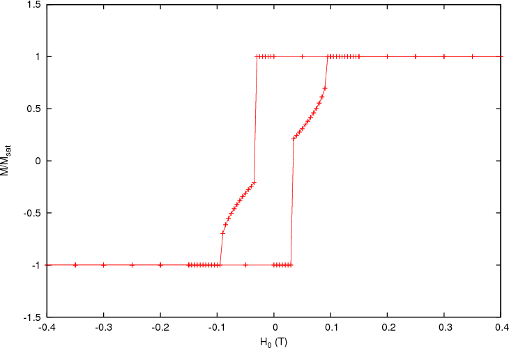
During the switching the system falls into an intermediate state, where the magnetisation is nearly aligned with the anisotropy easy axis.