2.27. Example: Parallel execution (MPI)
|Nmag|‘s numerical core (which is part of the |nsim| multi-physics library) has been designed to carry out numerical computation on several CPUs simultaneously. The protocol that we are using for this is the wide spread Message Passing Interface (MPI). There are a number of MPI implementations; the best known ones are probably MPICH1, MPICH2 and LAM-MPI. Currently, we support MPICH1 and MPICH2.
Which mpi version to use? Whether you want to use mpich1 or mpich2 will depend on your installation: currently, the installation from source provides mpich2 (which is also used in the virtual machines) whereas the Debian package relies on mpich1 (no Debian package is provided after release 0.1-6163).
2.27.1. Using mpich2
Before the actual simulation is started, a multi-purpose daemon must be started when using MPICH2.
The ``.mpd.conf`` file
MPICH2 will look for a configuration file with name .mpd.conf in
the user’s home directory. If this is missing, an attempt to start
the multi-purpose daemon, will result in an error message like
this:
$> mpd
configuration file /Users/fangohr/.mpd.conf not found
A file named .mpd.conf file must be present in the user's home
directory (/etc/mpd.conf if root) with read and write access
only for the user, and must contain at least a line with:
MPD_SECRETWORD=<secretword>
One way to safely create this file is to do the following:
  cd $HOME
  touch .mpd.conf
  chmod 600 .mpd.conf
and then use an editor to insert a line like
  MPD_SECRETWORD=mr45-j9z
into the file.  (Of course use some other secret word than mr45-j9z.)
If you don’t have this file in your home directory, just follow the
instructions above to create it with some secret word of your choice
(Note that the above example is from a Mac OS X system: on Linux the
home directory is usually under /home/USERNAME rather than
/Users/USERNAME as shown here.)
Let’s assume we have a multi-core machine with more than one CPU. This makes the mpi setup slightly easier, and is also likely to be more efficient than running a job across the network between difference machines.
First, we need to start the multi-purpose daemon:
$> mpd &
It will look for the file ~/.mpd.conf as described above. If found, it will start silently. Otherwise it will complain.
2.27.1.1. Testing that nsim executes in parallel
First, let’s make sure that nsim is in the search path. The command which nsim will return the location of the executable if it can be found in the search path. For example:
$> which nsim
/home/fangohr/new/nmag-0.1/bin/nsim
To execute nsim using two processes, we can use the command:
$> mpiexec -n 2 nsim
There are two useful commands to check whether nsim is aware of the intended MPI setup. The fist one is ocaml.mpi_status() which provides the total number of processes in the MPI set-up:
$> mpiexec -n 2 nsim
>>> ocaml.mpi_status()
MPI-status: There are 2 nodes (this is the master, rank=0)
>>>
The other command is ocaml.mpi_hello() and prints a short ‘hello’ from all processes:
>>> ocaml.mpi_hello()
>>> [Node   0/2] Hello from beta.kk.soton.ac.uk
[Node   1/2] Hello from beta.kk.soton.ac.uk
For comparison, let’s look at the output of these commands if we start nsim without MPI, in which case only one MPI node is reported:
$> nsim
>>> ocaml.mpi_status()
MPI-status: There are 1 nodes (this is the master, rank=0)
>>> ocaml.mpi_hello()
[Node   0/1] Hello from beta.kk.soton.ac.uk
Assuming this all works, we can now start the actual simulation. To
use two CPUs on the local machine to run the bar30_30_100.py
program, we can use:
$> mpiexec -n 2 nsim bar30_30_100.py
To run the program again, using 4 CPUs on the local machine:
$> mpiexec -n 4 nsim bar30_30_100.py
Note that mpich2 (and mpich1) will spawn more processes than there are
CPUs if necessary. I.e. if you are working on some Intel Dual Core
processor (with 2 CPUs and one core each) but request to run your
program with 4 (via the -n 4 switch given to mpiexec), than
you will have 4 processes running on the 2 CPUs.
If you want to stop the mpd daemon, you can use:
$> mpdallexit
For diagnostic purposes, the mpdtrace command can be use to track
whether a multipurpose daemon is running (and which machines are part
of the mpi-ring).
Advanced usage of mpich2
To run a job across different machines, one needs to start the
multi-purpose daemons on the other machines with the mpdboot
command. This will search for a file (in the current directory) with
name mpd.hosts which should contain a list of hosts to participate
(very similar to the machinefile in MPICH1).
To trace which process is sending what messages to the standard out,
one can add the -l switch to the mpiexec command: then each
line of standard output will be preceded by the rank of the process
who has issued the message.
Please refer to the official MPICH2 documentation for further details.
2.27.2. Using mpich1
Note: Most users will use MPICH2 (if they have compiled Nmag from the tar-ball): see Using mpich2
Suppose we would like to run Example 2: Computing the time development of a system of the manual with 2
processors using MPICH1. We need to know the full path to the nsim executable. In
a bash environment (this is pretty much the standard on Linux and
Mac OS X nowadays), you can find the path using the which
command. On a system where nsim was installed from the Debian package:
$> which nsim
/usr/bin/nsim
Let’s assume we have a multi-core machine with more than one CPU. This makes the mpi setup slightly easier, and is also likely to be more efficient than running a job across the network between difference machines. In that case, we can run the example on 2 CPUs using:
$> mpirun -np 2 /usr/bin/nsim bar30_30_100.py
where -np is the command line argument for the Number of Processors.
To check that the code is running on more than one CPU, one of the first few log messages will display (in addition to the runid of the simulation) the number of CPUs used:
$> mpirun -np 2 `which nsim` bar30_30_100.py

    nmag:2008-05-20 12:50:01,177   setup.py  269    INFO Runid (=name simulation) is 'bar30_30_100', using 2 CPUs
To use 4 processors (if we have a quad core machine available), we would use:
$> mpirun -np 4 /usr/bin/nsim bar30_30_100.py
Assuming that the nsim executable is in the path, and that we are
using a bash-shell, we could shortcut the step of finding the nsim
executable by writing:
$> mpirun -np 4 `which nsim` bar30_30_100.py
To run the job across the network on different machines simultaneously, we need to create a file with the names of the hosts that should be used for the parallel execution of the program. If you intend to use nmag on a cluster, your cluster administrator should explain where to find this machine file.
To distribute a job across machine1.mydomain,
machine2.mydomain, and machine3.mydomain we need to create the
file machines.txt with content:
machine1.mydomain
machine2.mydomain
machine3.mydomain
We then need to pass the name of this file to the mpirun command
to run a (mpi-enabled) executable with mpich:
mpirun -machinefile machines.txt -np 3 /usr/bin/nsim bar30_30_100.py
For further details, please refer to the MPICH1 documentation.
2.27.3. Visualising the partition of the mesh
We use Metis to partition the mesh. Partitioning means to allocate certain mesh nodes to certain CPUs. Generally, it is good if nodes that are spatially close to each other are assigned to the same CPU.
Here we demonstrate how the chosen partition can be visualised. As an example, we use the Example: demag field in uniformly magnetised sphere. We are Using mpich2:
$> mpd &
$> mpiexec -l -n 3 nsim sphere1.py
The program starts, and prints the chose partition to stdout:
 nfem.ocaml:2008-05-28 15:11:07,757    INFO Calling ParMETIS to partition the me
sh among 3 processors
 nfem.ocaml:2008-05-28 15:11:07,765    INFO Processor 0: 177 nodes
 nfem.ocaml:2008-05-28 15:11:07,765    INFO Processor 1: 185 nodes
 nfem.ocaml:2008-05-28 15:11:07,766    INFO Processor 2: 178 nodes
If you can’t find the information on the screen (=stdout), then have a
look in sphere1_log.log which contains a copy of the log messages
that have been printed to stdout.
If we save any fields spatially resolved (as with the
sim.save_data(fields='all') command), then nmag will create a file
with name (in this case) sphere1_dat.h5. In addition to the field
data that is saved, it also stores the finite element mesh in the
order that was used when the file was created. In this example, this
is the mesh ordered according to the output from the ParMETIS
package. The first 177 nodes of the mesh in this order are assigned to
CPU0, the next 185 are assigned to CPU1, and the next 178 are assigned to
CPU2.
We can visualise this partition using the nmeshpp command (which we
apply here to the mesh that is saved in the sphere1_dat.h5 file):
$> nmeshpp --partitioning=[177,185,178] sphere1_dat.h5 partitioning.vtk
The new file partitioning.vtk contains only one field on the mesh, and this has assigned to each mesh node the id of the associated CPU. We can visualise this, for example, using:
$> mayavi -d partitioning.vtk -m SurfaceMap
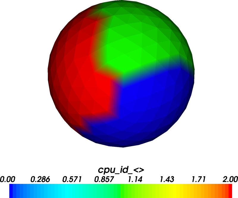
The figure shows that the sphere has been divided into three areas which carry values 0, 1 and 2 (corresponding to the MPI CPU rank which goes from 0 to 2 for 3 CPUs). Actually, in this plot we can only see the surface nodes (but the volume nodes have been partitioned accordingly).
The process described here is a bit cumbersome to visualise the
partition. This could in principle be streamlined (so that we save the
partition data into the _dat.h5 data file and can generate the
visualisation without further manual intervention). However, we expect
that this is not a show stopper and will dedicate our time to more
pressing issues. (User feedback and suggestions for improvements are
of course always welcome.)
2.27.4. Performance
Here is some data we have obtained on an IBM x440 system (with eight
1.9Ghz Intel Xeon processors). We use a test simulation (located in
tests/devtests/nmag/hyst/hyst.par) which computes a hysteresis
loop for a fairly small system (4114 mesh nodes, 1522 surface nodes,
BEM size 18MB). We use overdamped time integration to determine the
meta-stable states.
Both the setup and the time required to write data will not become significantly faster when run on more than one CPU. We provide:
total time: this includes setup time, time for the main simulation loop and time for writing data (measured in seconds)
total speedup: The speed up for the total execution time (i.e. ratio of execution time on one CPU to execution time on n CPUs).
sim time: this is the time spend in the main simulation loop (and this is where expect a speed up)
sim speedup: the speedup of the main simulation loop
| CPUs | total time | total speedup | sim time | sim speedup |
| 1 | 4165 | 1.00 | 3939 | 1.00 |
| 2 | 2249 | 1.85 | 2042 | 1.93 |
| 3 | 1867 | 2.23 | 1659 | 2.37 |
| 4 | 1605 | 2.60 | 1393 | 2.83 |
The numbers shown here have been obtained using mpich2 (and using the
ssm device instead of the default sock device: this is
available on Linux and resulted in a 5% reduction of execution time).
Generally, the (network) communication that is required between the nodes will slow down the communication. The smaller the system, the more communication has to happen between the nodes (relative to the amount of time spent on actual calculation). Thus, one expects a better speed up for larger systems. The performance of the network is also crucial: generally, we expect the best speed up on very fast networks and shared memory systems (i.e. multi-CPU / multi-core architectures). We further expect the speed-up to become worse (in comparison to the ideal linear speed-up) with an increasing number of processes.
2.28. Restarting MPI runs
There is one situation that should be avoided when exploiting parallel
computation. Usually, a simulation (involving for example a hysteresis
loop), can be continued using the --restart switch. This is also
true for MPI runs.
However, the number of CPUs used must not change between the initial
and any subsequent runs. (The reason for this is that the _dat.h5
file needs to store the mesh as it has been reordered for n CPUs. If
we continue the run with another number of CPUs, the mesh data will
not be correct anymore which will lead to errors when extracting the
data from the _dat.h5 file.)
Note also that there is currently no warning issued (in Nmag 0.1) if a user ventures into such a simulation.