2.6. Example: Vortex formation and propagation in disk

This example computes the evolution of a vortex in a flat cylinder magnetised along a direction orthogonal to the main axis.

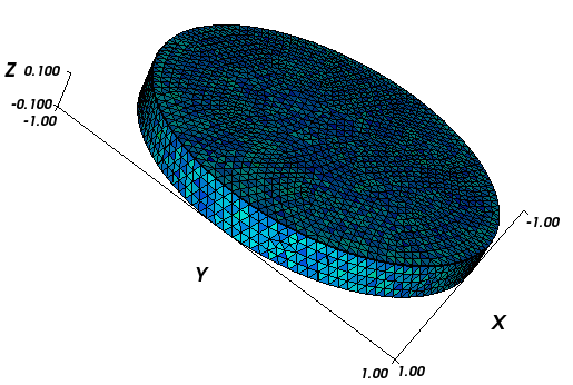
We use the same geometry as in the Hysteresis loop for thin disk example: a flat cylinder, 20 nm thick and 200 nm in diameter (the mesh is contained in nanodot.nmesh.h5):

To simulate the magnetised disc, we use the following script (nanodot.py):

import nmag
from nmag import SI, at

#create simulation object
sim = nmag.Simulation()

# define magnetic material
Py = nmag.MagMaterial( name="Py",
                       Ms=SI(795774,"A/m"),
                       exchange_coupling=SI(13.0e-12, "J/m")
                     )

# load mesh: the mesh dimensions are scaled by 100nm
sim.load_mesh( "../example_vortex/nanodot.nmesh.h5",
               [("cylinder", Py)],
               unit_length=SI(100e-9,"m")
             )

# set initial magnetisation
sim.set_m([1.,0.,0.])

Hs = nmag.vector_set( direction=[1.,0.,0.],
                      norm_list=[12.0, 7.0, [], -200.0],
                      units=1e3*SI('A/m')
                    )


# loop over the applied fields Hs
sim.hysteresis(Hs,
               save=[('averages', at('convergence')),
                     ('fields',   at('convergence')),
                     ('restart',  at('convergence')) 
                    ]
               )

We would like to compute the magnetisation behaviour in the applied fields ranging from [12e3, 0, 0] A/m to [-200e3, 0, 0] A/m in steps of -5e3 A/m. The command for this is:

Hs = nmag.vector_set( direction=[1,0,0],
                      norm_list=[12.0, 7.0, [], -200.0],
                      units=1e3*SI('A/m')
                    )

sim.hysteresis(Hs,
               save=[('averages', at('convergence')),
                     ('fields',   at('convergence')),
                     ('restart',  at('convergence'))
                    ]
              )

The ncol command allows us to extract the data and we redirect it to a text file with name nmag.dat:

$ ncol nanodot H_ext_0 m_Py_0 > nmag.dat

Plotting the data with `Gnuplot`_:

$ gnuplot make_comparison_plot.gnu

which uses the script in make_comparison_plot.gnu:

set term postscript eps enhanced color  
set out 'nanodot_evo.eps'
set xlabel 'Applied field (kA/m)'
set ylabel 'M / M_s'
plot [-250:50] [-1.2:1.2] 'magpar.dat' u 2:3 ti 'magpar' w lp 4 , 'nmag.dat' u ($1/1000):2  ti 'nmag' w lp 3

The resulting graph is shown here:

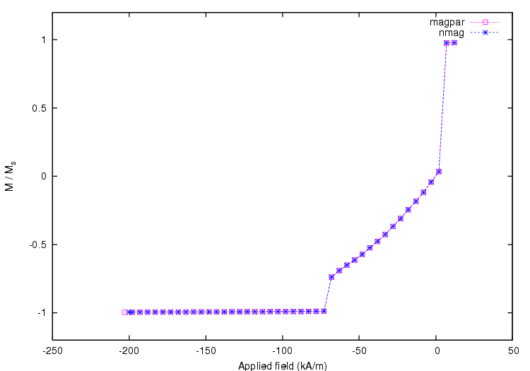
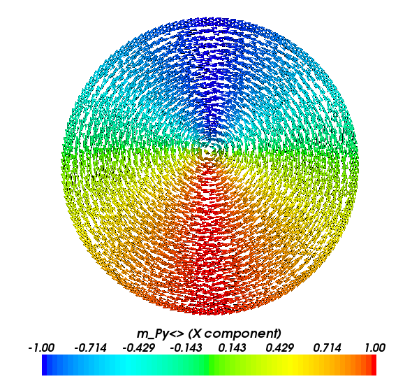
and we can see that the results from nsim match those from `magpar`_. The magnetisation configurations during the switching process are shown in the following snapshots:

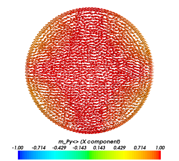
Magnetisation configuration for a decreasing applied field of 20 kA/m. The x-axis is increasing from left to right for this and the subsequent plots.

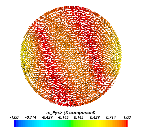
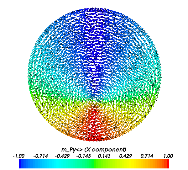
Magnetisation configuration for a decreasing applied field of 15 kA/m.

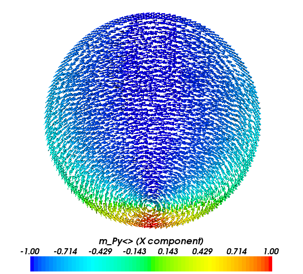
Magnetisation configuration for a decreasing applied field of 10 kA/m.

Magnetisation configuration for a decreasing applied field of -30 kA/m.

Magnetisation configuration for a decreasing applied field of -95 kA/m.

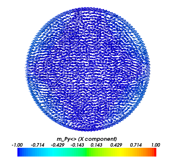
Magnetisation configuration for a decreasing applied field of -100 kA/m.

We see that during magnetisation reversal a vortex nucleates on the boundary of the disc when the field is sufficiently decreased from its saturation value. As the field direction is aligned with the x-axis, the vortex appears in the disc region with the largest y component, and it moves downwards towards the centre along the y-axis. With a further decrease of the applied field the vortex moves towards the opposite side of the disc with respect to the nucleation position, and it is eventually expelled when the magnetisation aligns with the field direction over all the disc.