2.25. Example: Calculation of dispersion curves¶

|Nmag| can be used to study the propagation of spin waves and to calculate dispersion curves. Here we consider a simulation script which shows how to do that. In particular, we study a long cylindrical wire made of Permalloy. We assume the magnetisation in the wire is relaxed along one axial direction (i.e. there are no domain walls inside the wire). One side of the wire is “perturbed” at time t=0 by a pulsed magnetic field. The spin waves generated on this side propagate towards the other. We want to study the propagation of spin waves and obtain the dispersion relation, i.e. a relation between the wave vector and the frequency of the spin-waves which propagate in the considered media. To calculate the dispersion relation we use the method developed by V. Kruglyak, M. Dvornik and O. Dmytriiev

In order to carry out such a numerical experiment, we first need to calculate the relaxed equilibrium magnetisation, i.e. the one which we perturb with the application of a pulsed field. Consequently, the simulation is split into two parts:

In part I, the system is relaxed to obtain the initial magnetisation configuration for zero applied field. Such a state is then saved into a file to be used in part II;
In part II, the magnetisation obtained in part I is loaded and used as the initial magnetisation configuration. A pulsed external magnetic field localised on one side of the wire is applied. The Landau-Lifshitz-Gilbert equation is integrated in time to compute the dynamical reaction to the applied stimulus. The configuration of the magnetisation is saved frequently to file, so that it can be studied and processed later.

The two parts are two simulations of the same system under different conditions. If we then decide to write two separate files for the two parts we end up duplicating the fragment of code which defines the materials and load the mesh. For this reason we split the simulation in three files:

"thesystem.py": defines the material which composes the nanowire and loads the mesh;
"relaxation.py": uses “thesystem.py” to setup the system and performs a relaxation with zero applied field. It saves the final magnetisation configuration to a file “m0.h5”;
"dynamics.py": uses “thesystem.py” to setup the system, loads the initial magnetisation configuration from the file “m0.h5” (produced by “relaxation.py”). It then applies a localised pulse of the applied magnetic field on one side of the wire and compute the dynamical response of the system saving the result to files.

Consequently, in order to run the full simulation the user will have to type two commands on the shell, one for each part of the simulation:

$ nsim relaxation.py
$ nsim dynamics.py

(there is no need to type nsim thesystem.py as this file is implicitly “included” by the other two). In the next sections we will go through the three files which make up the numerical experiment.

2.25.1. The system: `thesystem.py`¶

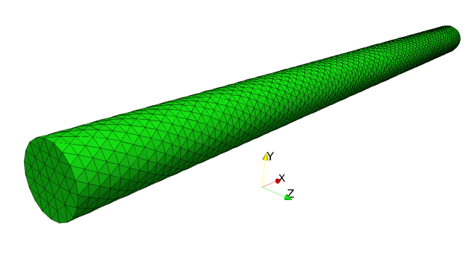
The system under investigation is a cylindrical nanopillar of radius r=3 nm and length l=600 nm. The mesh file cylinder.nmesh.h5 is obtained (using `Netgen`_). (The figure shows a cylinder that is 100nm long.)

The geometry file given to `Netgen`_ cylinder.geo is shown below:

    algebraic3d
    solid nanopillar = cylinder (-300.0, 0, 0; 300.0, 0, 0; 3.0)
                       and plane (-300.0, 0, 0; -1, 0, 0)
                       and plane ( 300.0, 0, 0;  1, 0, 0)
                       -maxh=1.0;
    tlo nanopillar;

The cylinder is made of Permalloy and as specified in the file thesystem.py shown below:

# In this file we define the material parameters and geometry of the system
# so that we can use it in two simulations: first during the relaxation,
# then during the dynamics

from nmag.common import *

nm = SI(1e-9, 'm')    # define nm as "nanometre"
ps = SI(1e-12, 's')   # define ps as "picosecond"

m0_filename = "m0.h5" # the file containing the equilibrium magnetisation

# A function which sets up the simulation with given name and damping
def simulate_nanowire(name=None, damping=0.5):
  permalloy = MagMaterial('Py',
                          Ms=SI(0.86e6, 'A/m'),
                          exchange_coupling=SI(13e-12, 'J/m'),
                          llg_damping=damping)

  s = Simulation(name)
  s.load_mesh("cylinder.nmesh.h5", [('nanopillar', permalloy)],
              unit_length=nm)
  return s

The file defines a few entities which are used in both the two parts of the simulations: nm is just an abbreviation for nanometer and similarly ps is an abbreviation for picosecond. m0_filename is the name of the file where the relaxed magnetisation will be saved (in part I) and loaded (in part II). Finally, the function simulate_nanowire deals with the portion of the setup which is common to both part I and part II. In particular, it defines a new material permalloy, creates a new simulation object s, load the mesh and associates to it the material permalloy. Such setup procedure is very similar to what has been encountered so far in the manual, the only element of novelty is that here we do it inside a function and return the created simulation object as a result of the function. The file defined here is not supposed to be run by itself, but rather to be used in part I and II.

2.25.2. Part I: `relaxation.py`¶

The source for the file relaxation.py is shown below:

# This script is used to compute the equilibrium configuration for the
# magnetisation, which is then used in the second part of the simulation,
# where the dynamics is actually studied.

from thesystem import simulate_nanowire, m0_filename, ps
from nmag.common import *

s = simulate_nanowire(name='relaxation', damping=0.5) # NOTE the high damping!
s.set_m([1, 0, 0])
s.relax(save=[('fields', at('time', 0*ps) | at('convergence'))])
s.save_restart_file(m0_filename)

The first two lines are used to import entities defined elsewhere. In particular, the first line in:

from thesystem import simulate_nanowire, m0_filename, ps
from nmag.common import *

tells to Python to load the file thesystem.py and “extract” from it the entities simulate_nanowire, m0_filename, ps. The second line does a similar thing and extracts all the quantities defined in the Nmag module nmag.common. This module defines some entities which are commonly used in simulations (such as every, at, SI, etc). The simulation is then set up using:

s = simulate_nanowire(name='relaxation', damping=0.5) # NOTE the high damping!

This line invokes the function simulate_nanowire, which does load the mesh and associate the material to it. The function returns the simulation object which is stored inside the variable s and is used in the following lines:

s.set_m([1, 0, 0])
s.relax(save=[('fields', at('time', 0*ps) | at('convergence'))])
s.save_restart_file(m0_filename)

Here we set the magnetisation along the axis of the nanopillar, we then relax the system to find the equilibrium magnetisation. We finally save such a configuration in the file m0_filename, i.e. with the name specified in thesystem.py.

2.25.3. Part II: `dynamics.py`¶

The source for the file dynamics.py is shown below:

from thesystem import simulate_nanowire, m0_filename, ps, nm
from nmag.common import *

# Details about the pulse
pulse_boundary = -300.0e-9 + 0.5e-9 # float in nm
pulse_direction = [0, 1, 0]
pulse_amplitude = SI(1e5, 'A/m')
pulse_duration = 1*ps

# Function which sets the magnetisation to zero
def switch_off_pulse(sim):
  sim.set_H_ext([0.0, 0.0, 0.0], unit=pulse_amplitude)

# Function which sets the pulse as a function of time/space
def switch_on_pulse(sim):
  def H_ext(r):
    if r[0] < pulse_boundary:
      return pulse_direction
    else:
      return [0.0, 0.0, 0.0]

  sim.set_H_ext(H_ext, unit=pulse_amplitude)

# Here we run the simulation: do=[....] is used to set the pulse
#   save=[...] is used to save the data.
s = simulate_nanowire('dynamics', 0.05)
s.load_m_from_h5file(m0_filename)
s.relax(save=[('fields', every('time', 0.5*ps))],
        do=[(switch_on_pulse, at('time', 0*ps)),
            (switch_off_pulse, at('time', pulse_duration)),
            ('exit', at('time', 200*ps))])

The simulation starts again importing a few entities from the file thesystem.py. In particular, the function simulate_nanowire is used to setup the system similarly to what was done for the relaxation. The next few lines define some variables which are used to define the geometry and duration of the magnetic field pulse:

# Details about the pulse
pulse_boundary = -300.0e-9 + 0.5e-9 # float in nm
pulse_direction = [0, 1, 0]
pulse_amplitude = SI(1e5, 'A/m')
pulse_duration = 1*ps

In this example the pulse is obtained by switching on the applied field (from (0, 0, 0) to (0, pulse_amplitude, 0)) in the region of the wire where x < pulse_boundary, which corresponds in this case to a layer of 0.5 nm thickness on one side of the cylinder. The pulse is switched on at t=0 and switched off at pulse_duration. We now examine the code and explain how all this is coded in the script. We start explaining the last few lines:

# Here we run the simulation: do=[....] is used to set the pulse
#   save=[...] is used to save the data.
s = simulate_nanowire('dynamics', 0.05)
s.load_m_from_h5file(m0_filename)
s.relax(save=[('fields', every('time', 0.5*ps))],
        do=[(set_pulse, at('time', 0*ps)),
            (set_to_zero, at('time', pulse_duration)),
            ('exit', at('time', 200*ps))])

Here we use the simulate_nanowire function which we defined in the file thesystem.py to setup the system and the materials. We then set the initial magnetisation configuration from the file saved in part I and carry out the time integration by calling the relax method of the simulation object s. The pulse is switched on and switched off by the instruction passed in the do=[...] argument. In particular, the argument do accepts a list of pairs (things to be done, at a given time). The code:

do=[(switch_on_pulse, at('time', 0*ps)),
    (switch_off_pulse, at('time', pulse_duration)),
    ('exit', at('time', 200*ps))]

specifies that:

the function switch_on_pulse should be executed at time t=0 ps;
the function switch_off_pulse should be executed at time t= pulse_duration;
the simulation should terminate at time t=200 ps.

At the same time the argument save=[('fields', every('time', 0.5*ps))] of the relax method saves the field every 0.5 ps.

Let’s now see how the pulse is actually switched on and off. To switch off the pulse we provide the function:

# Function which sets the magnetisation to zero
def switch_off_pulse(sim):
  sim.set_H_ext([0.0, 0.0, 0.0], unit=pulse_amplitude)

The function gets the simulation object, sim, as an argument and uses it together with the method set_H_ext to set the applied magnetic field to zero everywhere. The function to set up the simulation is a little bit more complicated:

# Function which sets the pulse as a function of time/space
def switch_on_pulse(sim):
  def H_ext(r):
    if r[0] < pulse_boundary:
      return pulse_direction
    else:
      return [0.0, 0.0, 0.0]

  sim.set_H_ext(H_ext, unit=pulse_amplitude)

Indeed, being the pulse localised (and hence non-uniform) in space, we need to define a function to be given to set_H_ext. The function checks whether the x component in the given point is lower than pulse_amplitude and sets the applied field to a value differt from zero only if that is really the case.

2.25.4. Postprocessing the data¶

Once the simulations are finished, the data (i.e. the values of the magnetisation saved every 0.5 ps) can be extracted from the file dynamics_dat.h5 and postprocessed. We use the nmagprobe command for this. nmagprobe can perform several postprocessing tasks (detailed documentation can be obtained by typing nmagprobe --help). In this context it is used to probe the magnetisation along the axis of the cylinder at regular intervals of time. The values extracted are then Fourier transformed. The command we use is the following:

nmagprobe --verbose dynamics_dat.h5 --field=m_Py \
  --time=0,100e-12,101 --space=-300,300,201/0/0 --ref-time=0.0 \
  --scalar-mode=component,1 --out=real-space.dat \
  --ft-axes=0,1 --ft-out=norm --ft-out=rec-space.dat

Here we extract data for the magnetisation (option --field=m_Py) from the file dynamics_dat.h5.

We probe the field over a cubic lattice in space and time. The lattice is four dimensional and consists of the points (t, x, y, z) with t=0, 1 ps, 2 ps, ..., 100 ps (101 values), x=-300 nm, -297 nm, -294 nm, ..., 300 nm (201 values) and y=z=0. The lattice is fully determined by the options --time and --space. In particular, the option --time=0,100e-12,101 states that the lattice consists of 101 equispaced values going from 0 to 100e-12 s. The option --space accepts a similar expressions for each spatial coordinate separated by /;
--ref-time=0.0 tells to nmagprobe that after extracting the values for the field, m(t, x, y, z), it should compute the difference with respect to the given time, i.e. dm(t, x, y, z) = m(t, x, y, z) - m(0, x, y, z). We add this option to nmagprobe because we are interested in the variation of the magnetisation with respect to the equilibrium configuration (t=0) rather than on its “absolute” value;
--scalar-mode=component,1 induces nmagprobe to extract the y component of dm and to use it as a scalar when writing the output and when doing the fourier transform (to extract the x component one should use --scalar-mode=component,0); We could also write --scalar-mode=component,y and --scalar-mode=component,x.
--out=real-space.dat induces nmagprobe to save to file the data selected by the options discussed so far. In particular, the file real-space.dat will be filled with the values of the y-component of dm(t, x, y, z) along the selected lattice. That will be a text file which can be inspected with a text editor and used within plotting programs such as `Gnuplot`_;
--ft-axes=0,1 specifies that the selected data should be Fourier transformed along the axis 0 (time) and 1 (x-space). This can also be written as --ft-axes=t,x.
--ft-out=norm induces nmagprobe to compute the norm of the complex numbers coming from the Fourier-transform. These are the values which are finally saved to file;
--ft-out=rec-space.dat specifies the output file for the Fourier-transformed data.

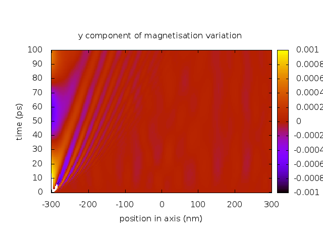
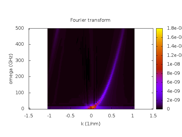
The command creates two files: real-space.dat, containing the y component of the magnetisation variation as a function of time and space, and rec-space.dat, containing the Fourier transform of such a quantity.

To plot the data in the two files we use the `Gnuplot`_ script plot.gnp:

set term png
set pm3d map

set out "real-space.png"
set title "y component of magnetisation variation"
set xlabel "position in axis (nm)"
set ylabel "time (ps)"
splot [] [0:] [-0.001:0.001] 'real-space.dat' u ($2):($1/1e-12):5 t ""

set out "rec-space.png"
set title "Fourier transform"
set xlabel "k (1/nm)"
set ylabel "omega (GHz)"
splot [] [0:] [0:1.7e-8] 'rec-space.dat' u (-$2):($1/(2*pi*1e9)):5 t ""

Here is the result after running the script with Gnuplot.

2.25. Example: Calculation of dispersion curves¶

2.25.1. The system: thesystem.py¶

2.25.2. Part I: relaxation.py¶

2.25.3. Part II: dynamics.py¶

2.25.4. Postprocessing the data¶

2.25.1. The system: `thesystem.py`¶

2.25.2. Part I: `relaxation.py`¶

2.25.3. Part II: `dynamics.py`¶