2.22. Example: Current-driven magnetisation precession in nanopillars
This is the second example we provide in order to illustrate the usage of the Zhang-Li extension to model spin-transfer-torque in |Nmag|. While in the Current-driven motion of a vortex in a thin film example we tried to present two scripts (one for initial relaxation, and one for the spin torque transfer simulation), sacrificing usability for the sake of clarity, here we’ll try to present a real-life script, using the power of the Python programming language as much as it is needed to achieve our goal.
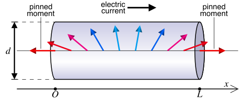
We consider a ferromagnetic nanopillar in the shape of a cylinder. We assume that the magnetisation in the nanopillar is pinned in the two faces of the cylinder along opposite directions: on the right face the magnetisation points to the right, while on the left face it points to the left. The magnetisation is then forced to develop a domain wall. We then study how such an “artificial” domain wall interacts with a current flowing throughout the cylinder, along its axis.
By “artificial” we mean that the domain wall is developed as a consequence of the pinning, which we artificially impose. In real systems, the pinning can be provided through interface exchange coupling or may have a geometrical origin, in combination with suitable material parameters. The situation we consider here is described and studied in more detail in publications [1] and [2].
| [1] | (1, 2) Matteo Franchin, Thomas Fischbacher, Giuliano Bordignon, Peter de Groot, Hans Fangohr, Current-driven dynamics of domain walls constrained in ferromagnetic nanopillars, Physical Review B 78, 054447 (2008), online at http://eprints.soton.ac.uk/59253, |
| [2] | (1, 2) Matteo Franchin, Giuliano Bordignon, Peter A. J. de Groot, Thomas Fischbacher, Jurgen P. Zimmermann, Guido Meier, Hans Fangohr, Spin-polarized currents in exchange spring systems, Journal of Applied Physics 103, 07A504 (2008), online at http://link.aip.org/link/?JAPIAU/103/07A504/1 |
2.22.1. Two simulations in one single script
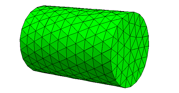
The nanopillar is made of Permalloy and has the shape of a cylinder with
radius of 10 nm and length 30 nm. The mesh is loaded from the file
l030.nmesh.h5
which was created using `Netgen`_ from the file
l030.geo.
The simulation is subdivided into two parts, similarly to the previous example:
- In part I, the system is relaxed to obtain the initial magnetisation configuration when the current is not applied.
- In part II the current is applied to the artificial domain wall whose shape was calculated in part I.
This time, however, we use just one single script to execute both parts of the simulation in one go. In particular, we define a function which takes some input parameters such as the current density, the damping, etc and uses them to carry out a simulation. We then call this function twice: once for part I and once for part II.
The full listing of the script stt_nanopillar.py:
import nmag, os, math
from nmag import SI, every, at
from nsim.si_units.si import degrees_per_ns

l = 30.0                        # The nanopillar thickness is 30 nm
hl = l/2                        # hl is half the nanopillar thickness
relaxed_m_file = "relaxed_m.h5" # File containing the relaxed magnetisation
mesh_name = "l030.nmesh.h5"     # Mesh name
mesh_unit = SI(1e-9, "m")       # Unit length for space used by the mesh

def run_simulation(sim_name, initial_m, damping, stopping_dm_dt,
                   j, P=0.0, save=[], do=[], do_demag=True):
  # Define the material
  mat = nmag.MagMaterial(
          name="mat",
          Ms=SI(0.8e6, "A/m"),
          exchange_coupling=SI(13.0e-12, "J/m"),
          llg_damping=damping,
          llg_xi=SI(0.01),
          llg_polarisation=P)

  # Create the simulation object and load the mesh
  sim = nmag.Simulation(sim_name, do_demag=do_demag)
  sim.load_mesh(mesh_name, [("np", mat)], unit_length=mesh_unit)

  # Set the pinning at the top and at the bottom of the nanopillar
  def pinning(p):
    x, y, z = p
    tmp = float(SI(x, "m")/(mesh_unit*hl))
    if abs(tmp) >= 0.999:
      return 0.0
    else:
      return 1.0
  sim.set_pinning(pinning)

  if type(initial_m) == str:            # Set the initial magnetisation
    sim.load_m_from_h5file(initial_m)   # a) from file if a string is provided
  else:
    sim.set_m(initial_m)                # b) from function/vector, otherwise

  if j != 0.0:                          # Set the current, if needed
    sim.set_current_density([j, 0.0, 0.0], unit=SI("A/m^2"))

  # Set additional parameters for the time-integration and run the simulation
  sim.set_params(stopping_dm_dt=stopping_dm_dt,
                 ts_rel_tol=1e-7, ts_abs_tol=1e-7)
  sim.relax(save=save, do=do)
  return sim

# If the initial magnetisation has not been calculated and saved into
# the file relaxed_m_file, then do it now!
if not os.path.exists(relaxed_m_file):
  # Initial direction for the magnetisation
  def m0(p):
      x, y, z = p
      tmp = min(1.0, max(-1.0, float(SI(x, "m")/(mesh_unit*hl))))
      angle = 0.5*math.pi*tmp
      return [math.sin(angle), math.cos(angle), 0.0]

  save = [('fields', at('step', 0) | at('stage_end')),
          ('averages', every('time', SI(5e-12, 's')))]

  sim = run_simulation(sim_name="relaxation", initial_m=m0,
                       damping=0.5, j=0.0, save=save,
                       stopping_dm_dt=1.0*degrees_per_ns)
  sim.save_restart_file(relaxed_m_file)
  del sim

# Now we simulate the magnetisation dynamics
save = [('averages', every('time', SI(9e-12, 's')))]
do   = [('exit', at('time', SI(6e-9, 's')))]
run_simulation(sim_name="dynamics", initial_m=relaxed_m_file, damping=0.02,
               j=0.1e12, P=1.0, save=save, do=do, stopping_dm_dt=0.0)
After importing the required modules, we define some variables such as
the length of the cylinder, l; the name of the file where to put
the relaxed magnetisation, relaxed_m_file; the name of the mesh,
mesh_name; its unit length, mesh_unit:
l = 30.0                        # The nanopillar thickness is 30 nm
hl = l/2                        # hl is half the nanopillar thickness
relaxed_m_file = "relaxed_m.h5" # File containing the relaxed magnetisation
mesh_name = "l030.nmesh.h5"     # Mesh name
mesh_unit = SI(1e-9, "m")       # Unit length for space used by the mesh
These quantities are used later in the script. For example, knowing the length of the nanopillar is necessary in order to set a proper initial magnetisation for the relaxation. By making this a parameter at the top of the program, we can change it there (if we wan to study the same system for a different l), and just run the script again.
We define the function run_simulation: we teach Python how to run
a simulation given some parameters, such as the initial magnetisation,
the damping, the current density, etc. The function is defined
starting with the line:
def run_simulation(sim_name, initial_m, damping, stopping_dm_dt,
                   j, P=0.0, save=[], do=[], do_demag=True):
The arguments of the function (the names inside the parenthesis) are
those parameters which must be choosen differently in part I and part II.
For example, we decided to make the current density j an argument
for the function run_simulation, because in part I j must be set
to zero, while in part II it must be set to some value greater than zero.
On the other hand, the saturation magnetisation does not appear
in the argument list of the function, since it has the same value
both in part I and part II.
A remark about the Python syntax: arguments such as sim_name
must be specified explicitly when using the function run_simulation,
while arguments such as P=0 have a default value (0.0 in this case)
and the user may omit them, meaning that Python will then use
the default values.
We skip the explanation of the body of the function and focus on the code which
follows it. We’ll return later on the implementation of run_simulation.
For now, the user should keep in mind that run_simulation just runs
one distinct micromagnetic simulation every time it is called (and what simulation this is will depend on the parameters given to the function). The function returns
the simulation object which it created.
We now comment the code which follows the function run_simulation:
# If the initial magnetisation has not been calculated and saved into
# the file relaxed_m_file, then do it now!
if not os.path.exists(relaxed_m_file):
  # Initial direction for the magnetisation
  def m0(pos):
      x, y, z = pos
      tmp = min(1.0, max(-1.0, float(SI(x, "m")/(mesh_unit*hl))))
      angle = 0.5*math.pi*tmp
      return [math.sin(angle), math.cos(angle), 0.0]

  save = [('fields', at('step', 0) | at('stage_end')),
          ('averages', every('time', SI(5e-12, 's')))]

  sim = run_simulation(sim_name="relaxation", initial_m=m0,
                       damping=0.5, j=0.0, save=save,
                       stopping_dm_dt=1.0*degrees_per_ns)
  sim.save_restart_file(relaxed_m_file)
  del sim
This piece of code carries out part I of the simulation: it relaxes the system starting from a sensible initial guess for the magnetisation and saves the relaxed magnetisation configuration so that it can be used in part II.
In more detail, it starts by checking (using the function
os.path.exists) if a file containing the initial magnetisation
exists. If this is not the case, then the following indented block
will be executed, which computes and saves this initial
magnetisation. If the file exists, the whole indented block is
skipped, and we go straight to part II of the calculation.
In order to compute the relaxed configuration, an initial guess m0
for the magnetisation is defined. Such magnetisation linearly rotates
from left to right as the position changes from the left face to the
right face of the cylinder. Here x is the x coordinate of the
position vector p and tmp = min(1.0, max(-1.0, float(SI(x,
"m")/(mesh_unit*hl)))) is a continuous function which changes
linearly from -1 to 1 when going from the left to the right face,
keeping constant outside the cylinder.
In the code above we also define the variable save which is used
to specify when and what should be saved to disk. Here we save the
fields before and after the relaxation and save the averages every 5
picoseconds.
We then call the run_simulation function we defined above to relax
the magnetisation. This function returns the simulation object
sim, which we use to save the magnetisation using the
save_restart_file function.
Once this is done, we delete the simulation object, releasing resources
(memory) we have used for the simulation of part I. Note that for
the relaxation, we use j=0.0 (zero current density), damping=0.5
(fast damping, to reach convergence quickly) and
stopping_dm_dt=1.0*degrees_per_ns (this means that the simulation
should end when the magnetisation moves slower than 1 degree per
nanosecond).
The following part of the script deals with part II, the computation of the current-driven dynamics:
# Now we simulate the magnetisation dynamics
save = [('averages', every('time', SI(9e-12, 's')))]
do   = [('exit', at('time', SI(6e-9, 's')))]

run_simulation(sim_name="dynamics",
               initial_m=relaxed_m_file,
               damping=0.02,
               j=0.1e12,
               P=1.0,
               save=save,
               do=do,
               stopping_dm_dt=0.0)
Here we decide to save the averages every 9 picoseconds and exit the
simulation after 6 nanoseconds. We use stopping_dm_dt=0.0 to
disable the convergence check (here we just want to simulate for a
fixed amount of time). We also use full spin polarisation, P=1.0,
we apply a current density of j=0.1e12 A/m^2 and use a realistic
damping parameter for Permalloy, damping=0.02. For the initial
magnetisation we pass the name of the file where the relaxed
magnetisation was saved in part I and we specify a simulation name
sim_name="dynamics" which is different from the one used for the
relaxation (which was sim_name="relaxation"). The simulation name
will decide the prefix of any filenames that are being created when
saving data. (If the simulation name is not specified, the name of the
script file is used.)
We now return to discuss the function run_simulation and see how
it carries out the actual simulations. First, the function defines the
material:
# Define the material
mat = nmag.MagMaterial(
        name="mat",
        Ms=SI(0.8e6, "A/m"),
        exchange_coupling=SI(13.0e-12, "J/m"),
        llg_damping=damping,
        llg_xi=SI(0.01),
        llg_polarisation=P)
It uses the variable P which is passed as an argument to the function.
Then the simulation object is created and the mesh is loaded:
# Create the simulation object and load the mesh
sim = nmag.Simulation(sim_name, do_demag=do_demag)
sim.load_mesh(mesh_name, [("np", mat)], unit_length=mesh_unit)
Note that sim_name is passed to the Simulation object,
allowing the user to use different prefixes for the output files
of the simulation. For example, if sim_name = "relaxation",
then the output files produced when saving the fields or their averages
to disk will have names starting with the prefix relaxation_.
On the other hand, if sim_name = "dynamics", the names of these files
will all start with the prefix dynamics_.
Using different simulation names allows us to save the data of part I and part II in different independent files. The function continues with the code above:
# Set the pinning at the left and right face of the nanopillar
def pinning(p):
  x, y, z = p
  tmp = float(SI(x, "m")/(mesh_unit*hl))
  if abs(tmp) >= 0.999:
    return 0.0
  else:
    return 1.0
sim.set_pinning(pinning)
which is used to pin the magnetisation at the left and right faces of
the cylinder. Note here that x is the x component of the position
of the mesh site and that:
tmp = float(SI(x, "m")/(mesh_unit*hl))
is equal to -1 at the right face, and to +1 at the left face.
We then set the magnetisation. If initial_m is a string,
then we assume it is the name of the file and load the magnetisation
with the method load_m_from_h5file, otherwise we assume it is just
a function and set the magnetisation in the usual way, using the method
set_m:
if type(initial_m) == str:            # Set the initial magnetisation
  sim.load_m_from_h5file(initial_m)   # a) from file if a string is provided
else:
  sim.set_m(initial_m)                # b) from function/vector, otherwise
We then set the current density along the x direction
(only if j is not zero):
if j != 0.0:                          # Set the current, if needed
  sim.set_current_density([j, 0.0, 0.0], unit=SI("A/m^2"))
Finally, we set tolerances, the stopping criterion and launch the simulation:
# Set additional parameters for the time-integration and run the simulation
sim.set_params(stopping_dm_dt=stopping_dm_dt,
               ts_rel_tol=1e-7, ts_abs_tol=1e-7)
sim.relax([None], save=save, do=do)
return sim
The relax function carries out the simulation, taking into account the stopping criterion and save and do actions. Finally, the function returns the simulation object which it created.
2.22.2. Results: precession of the magnetisation
We launch the script with:
$ nsim stt_nanopillar.py
The script runs both part I (output files starting with relaxation_)
and part II (output files starting with dynamics_).
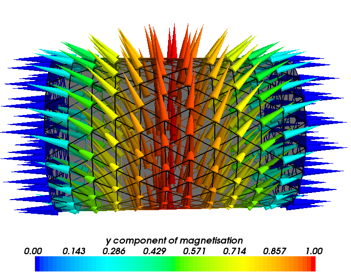
The relaxed magnetisation can be extracted and saved into a vtk file using
the command nmagpp relaxation --vtk=m.vtk. MayaVi can then be used
to obtain the following picture:
We can now take a look at the results obtained for the dynamics. The average magnetisation as a function of time can be extracted using:
ncol dynamics time M_mat_0 M_mat_1 M_mat_2 > m_of_t.dat
We can use the following gnuplot script:
set term postscript color eps enhanced solid
set out "m_of_t.eps"

set xlabel "time (ns)"
set ylabel "average magnetisation (10^6 A/m)"
plot [0:6] \
  "m_of_t.dat" u ($1*1e9):($2/1e6) t "<M_x>" w l, \
  "" u ($1*1e9):($3/1e6) t "<M_y>" w l, \
  "" u ($1*1e9):($4/1e6) t "<M_z>" w l
and obtain the following graph:
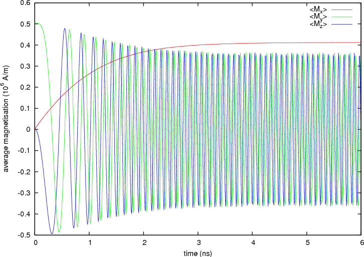
The sinusoidal dependence of the y and z magnetisation components suggests that the magnetisation rotates around the nanopillar axis with a frequency which increases to approach its maximum value.
A more detailed discussion of results and interpretation is provided in the publications [1] and [2] mentioned in section Example: Current-driven magnetisation precession in nanopillars.